Material
- Metallic Materials Properties Development and Standardization (MMPDS-2024)
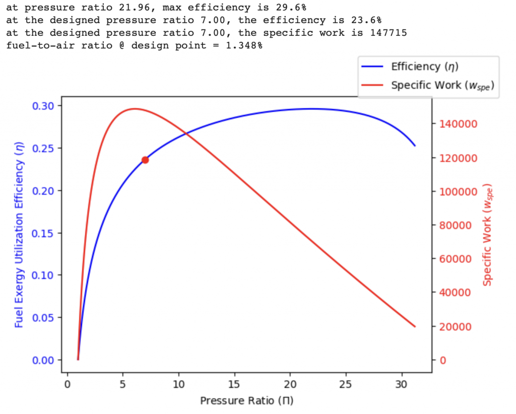
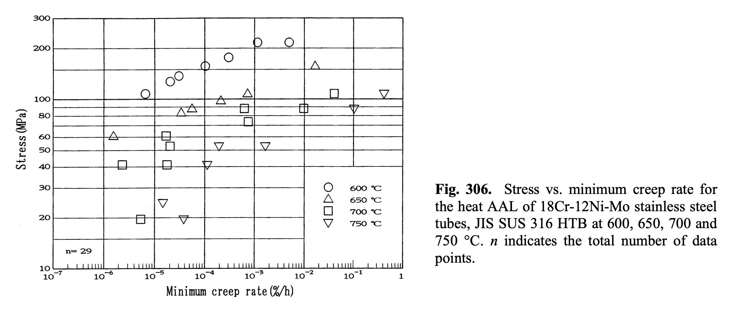
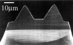
The design target for the second generation engine is a power output of 10 kW with a thermal efficiency, defined as the equation below, of more than 10%. $$ \eta_\textrm{thermal}=\frac{\text{net power out}}{\text{fuel mass flow rate} \times \text{fuel lower heating value}}=\frac{(1+f)c_p^c T_{t4} \eta_T (1-\Pi^{\frac{1-\gamma^c}{\gamma^c}}) – \frac{c_p^a T_{0}}{\eta_C} (\Pi^{\frac{\gamma^a-1}{\gamma^a}}-1)}{f h_c} $$ For ease of fabrication, the turbine material is selected to be 316 Stainless Steel, which has a yield strength of more than 120 MPa at 650 C. For long term exposure to heat, it has less than 0.1% elongation at 1000 hours at 85 MPa at 650 C [1]. This decision leads to $T_{t4}=650 \text{ C} \approx 920 \text{ K}$.
The second generation engine is expected to have a radial compressor and an axial turbine. A conservative estimation of compressor efficiency and turbine efficiency is made: $\eta_c = 0.8$, $\eta_t = 0.85$.
The fuel is selected to be propane, which has a lower heating value of $h_c = 4.64 \times 10^7$ J / kg.
Some common assumptions are made to the rest of the variables:
Now, plotting $\eta_\textrm{thermal}$ vs pressure ratio $\Pi$ using this code, we have 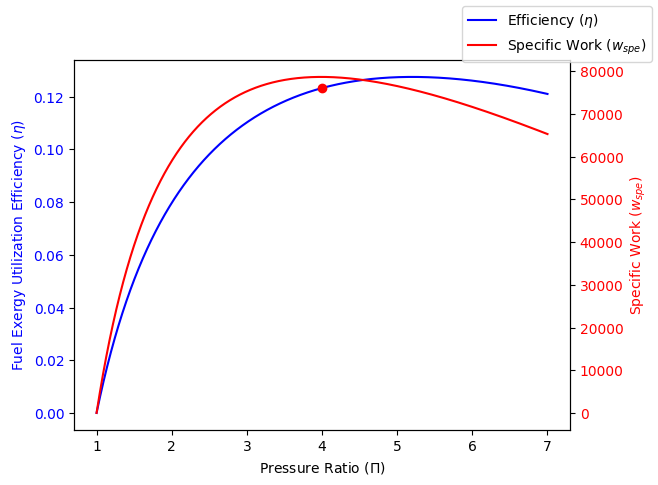
The pressure ratio is set to 4.0 to maximize specific work. At this design point, specific work is 78,700 J/kg and $\eta_\textrm{thermal}$ is predicted to be 12.3%. Fuel-to-air ratio at design point is calculated as $$f = \frac{c^c_p T_{t4} – c_p^a T_{t3}}{h_c-c_p^c T_{t4}}= 1.376%$$, where $T_{t3}$ is calculated as $$T_{t3} = T_0 (\frac{\Pi^{(\gamma^a-1)/\gamma^a}-1}{\eta_c}+1) = 479 \text{ K}$$.
According to specific work, in order to have 10 kW output, we need a massflow rate of 0.127 kg/s. This is less than half of the massflow rate designed for Gentoo. Due to a previous calculation error, a massflow rate of 0.128 kg/s will be used for the rest of the documents.
Aiming for a compact size, to get to this kind of pressure ratio is almost required to go with hybrid or full ceramic bearings. A very cost effective choice is this hybrid ceramic bearing from GRW, which is rated at 160,000 rpm. So, let’s set the upper limit of spool speed to 160,000 rpm. Other bearing choices for this speed would be: CXMC-1980 and HY KH 61900 C TA.
Due to the limitation of fabrication equipment, we can process rod stock with a diameter up to 200 mm. Say, half of the diameter is reserved for diffuser, the impeller diameter $D_w \leq 100$ mm.
As a summary, the following design requirements are selected for the impeller:
According to [3, p. 326], it is common to pick a flow coefficient in the range of $0.07 \leq \phi_{t1} \leq 0.10$. See the figure below (quoted from the book) for the relationship. Originally, a $\phi_{t1} = 0.09$ is selected for highest efficiency. But later, $\phi_{t1} = 0.057$ is used due the speed limitation imposed by bearings.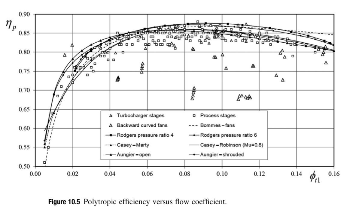
According to multiple source, it is common to have a work coefficient around 0.7 for higher efficiency and lower tip speed. Therefore, work coefficient is choosen to be $\lambda = \frac{c_{u2}}{u_2} = \frac{\Delta h_t}{(\omega R_2)^2} = \frac{\omega \Delta (rc\theta)}{(\omega R_2)^2} = 0.7$.
According to [3, p. 330], We have:
$$ M_{u2}^2=\frac{\Pi^{\frac{\gamma-1}{\eta_{\text{ploy}} \cdot \gamma}}-1}{(\gamma-1)\lambda} $$
According to the definition of polytropic efficiency and assumption for ideal gas, we have
$$ \eta_c = \frac{\Pi^{(\gamma-1)/\gamma}-1}{\Pi^{(\gamma-1)/(\eta_{\text{poly}}\gamma)}-1} $$
Therefore, we have
$$ M_{u2}^2 = \frac{\Pi^{(\gamma-1)/\gamma}-1}{\eta_c(\gamma-1)\lambda} \approx 2.17 $$
and
$$ M_{u2} \approx 1.473 $$
Therefore,
$$ u_2=M_{u2}\sqrt{\gamma \text{R} T_{0}} \approx 510 \text{ m/s} $$
This result matches the prediction in [3, p. 267]. The Diameter of the impeller can be then calculated as (from [3, p. 255]):
$$ D_2 = \sqrt{\frac{\dot{m}}{\rho_{t1}u_2\phi_{t1}}} $$
When using $\rho_{t1}=1.18$ kg/m$^3$, we have $D_2$ = 61.1 mm. The speed is then calculated to be $\omega$ = 159,315 rpm. Both $D_2$ and $\omega$ satisfy our design requirements.
Then the relative Mach number at the inlet tip can be calculated as
$M_{w1}=\frac{M_{u2}(\frac{3.2 \phi_{t1}}{k})^{0.36}}{1-0.15M_{u2}(0.45+\frac{\phi_{t1}}{k})} = 0.931$, where impeller inlet shape factor $k = 1-(\frac{r_{1h}}{r_{1c}})^2 = 0.91$ is assumed. Equation source: [3, p. 353].
Then optimal flow inlet angle can be calculated as $\beta_{1c}=cos^{-1}(\frac{\sqrt{3+\gamma M_{w1}^2 + 2 M_{w1}} – \sqrt{3+ \gamma M_{w1}^2-2M_{w1}}}{2M_{w1}})=1.047 \text{ rad}= 60.0 ^\circ $. Source: [3, p 348].
The inlet diameter ratio can be then calculated as $\frac{D_{1c}}{D_2}= \frac{M_{w1}\sin (\beta_{1c})}{M_{u2}\sqrt{1+\frac{\gamma -1}{2}M_{w1}^2 \cos ^2{\beta_{1c}}}}=0.536 $ . Source: [4].
Then we know our impeller eye diameter $D_{1c}=32.8 $ mm. After that, inlet hub diameter can be calculated using inlet shape diameter $k$, $D_{1h}=D_{1c}\sqrt{1-k}=9.8 $ mm.
Impeller relative velocity at the casing can be then calculated as $w_{1c} = u_2 \frac{2D_{1c}}{\sqrt{3}D_2} = 316 $ m/s.
A de Haller number of $\text{DH} = 0.6$ is choose for medium diffusion. Then $w_2= \text{DH} \cdot w_{c1}=190$ m/s.
By ultilizating, outlet velocity triangle, $\frac{w_{u2}-c_s}{c_{m2}}=\tan \beta_2’ $ and the Wiesner correlation $\frac{c_s}{u_2}=\frac{\sqrt{\cos \beta_2’}}{Z^{0.7}}$ where Z is the number of blades at outlet, we can solve for the outlet backsweep angle $\beta_2’=26.8 ^\circ$ if $Z = 10$, or $\beta_2’=32.0 ^\circ$ if $Z = 12$, or $\beta_2’=35.5 ^\circ$ if $Z = 14$. In order to have a high efficiency and side operating range, $Z = 12$ is chosen for a backsweep angle of $\beta_2’=32.0 ^\circ$.

(Figure Source: [3])
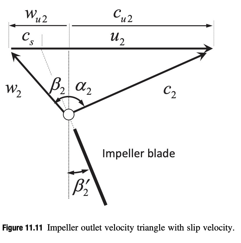
(Figure & Estimation Source: [3]. See section 11.6.6 in this book for outlet velocity triangle design process.)
The pressure rise coefficient $\psi=\frac{\Delta h_0}{U^2}=\frac{\Delta p}{\rho \omega^2D_2^2}=\lambda\eta_s=0.56$. According to [3, p. 285], an optimal value of $\psi=0.55 \pm 0.05$ is recommended. Our $\psi$ is in the optimal range.
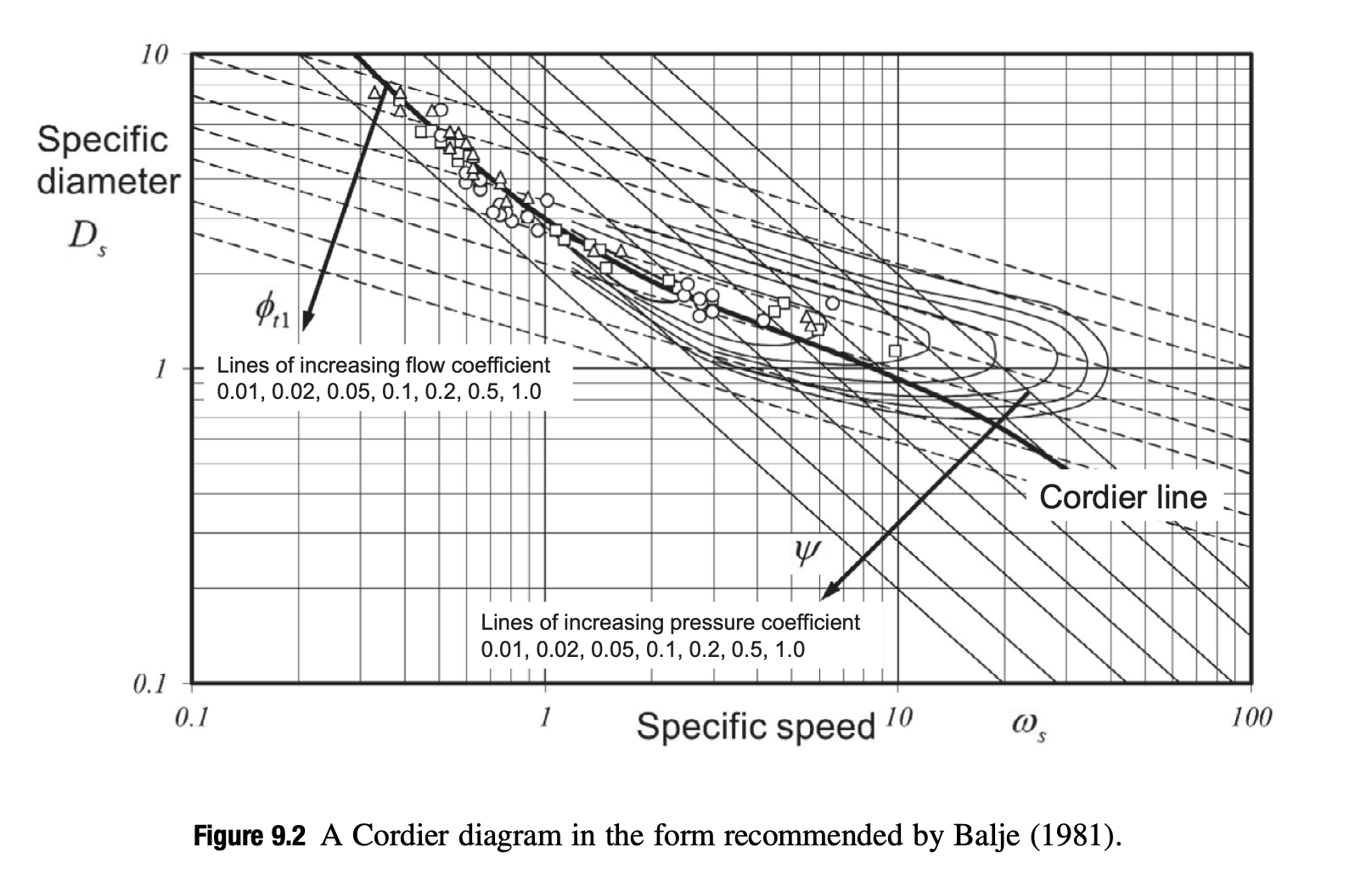
Then specific speed is calculated as $\omega_s=2\frac{\phi_{t1}^{1/2}}{\psi^{3/4}}=0.7376$, while the specific diameter is calculated as $D_s = \frac{\psi^{1/4}}{\phi_{t1}^{1/2}} = 3.623 $.
According to a cordier diagram plotted in [3, p. 291], our design point is very close to the Cordier Line (max efficiency).
An axial turbine configuration rather than radial turbine is selected for higher efficiency. Since the pressure ratio of compressor is only 4, single stage axial turbine should be able to do the work with fairly high efficiency.
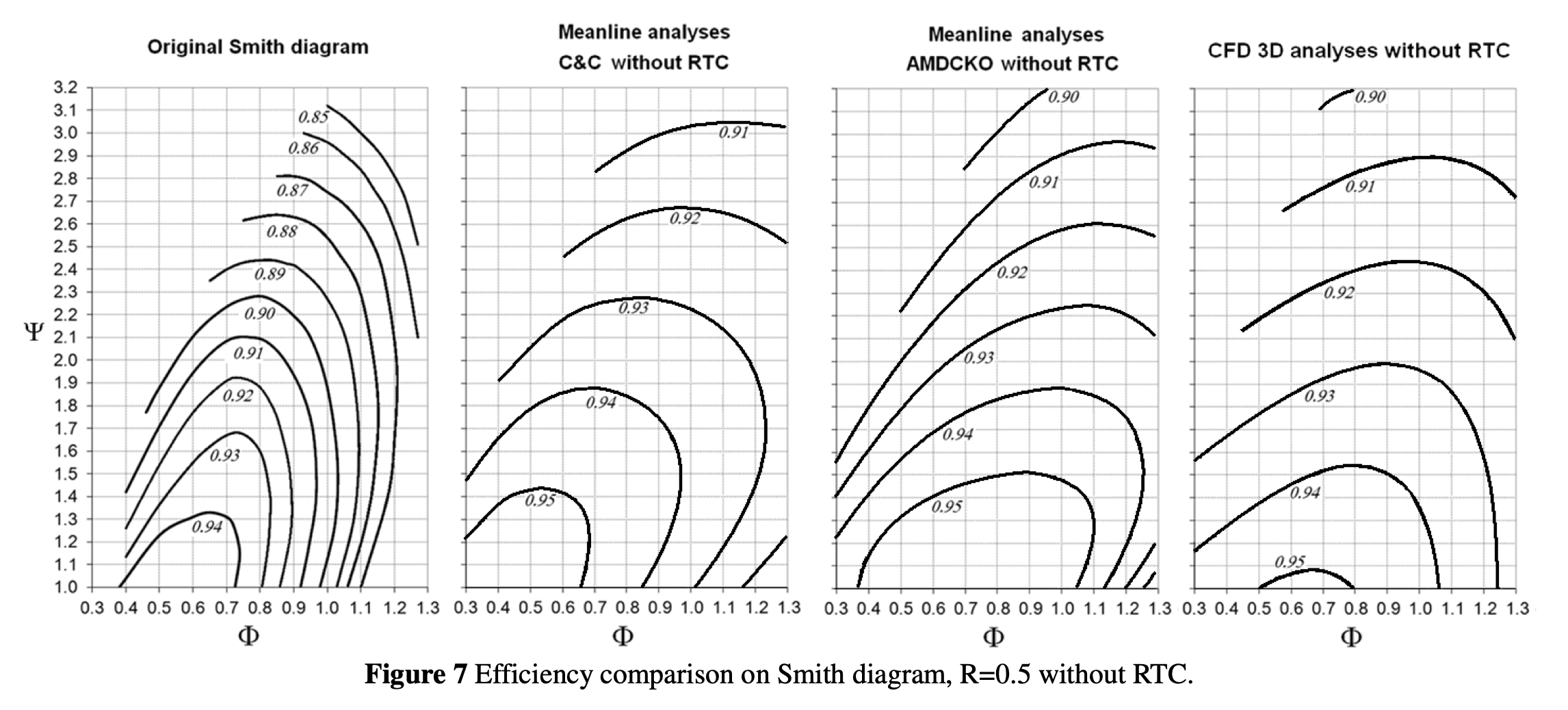
Multiple versions of Smith Charts are avaliable to help select these parameters. The following values are selected for maximum efficiency:
The following parameter is a bit away from optimal due to the stress consideration imposed by turbine material:
The defination of these parameter can be found at [6, p. 122-123].
A recommanded paper about Smith Chart can be found in [7]. Here’s one version of Smith Chart from this paper:
The turbine will be installed on the same shaft with compressor impeller, and therefore $\omega_t = \omega_c = $ 159,315 rpm.
The turbine should be able to supply the right amount of power to run compressor. From the compressor design, the compressor need a specific work of
$$ W_{sp}= \frac{c_p^a T_{0}}{\eta_c} (\Pi^{\frac{\gamma^a-1}{\gamma^a}}-1)= \text{181,757 J/kg} $$
Assuming there’s a 1% mechanical loss, suggested in [8, p. 65], the turbine needs to extract $W_{sp}= $ 183,593 J/kg. Therefore, the power needed to run the compressor is $23.5$ kw.
Then the pressure ratio needed for the turbine to provide enough power can be calculated as $$ \Pi_{\text{turbine}}=(1-\frac{W_{sp}}{(1+f)c_p^c T_{t4} \eta_T })^{\frac{\gamma^c}{1-\gamma^c}} = 2.53 $$
According to [8, p. 134], minimal blade tip speed can be calculated as $$ U \geq \sqrt{\frac{\dot{W}}{\dot{m}\Psi}}=391.1 \text{ m/s} $$ Using air density $\rho=1.53$ kg/m$^3$ at 4 atm pressure and 650 C, the annulus area can be calculated as $$ A_x=\frac{\dot{m}}{\rho\phi U}=237.7 \text{ mm}^2 $$ By using the equation $$ A_x=\pi r_t^2(1-(\frac{r_h}{r_t})^2) $$ and the following equation from [8, p. 152]. which estimates centrifugal stress $$ \frac{\sigma_c}{\rho_m}=\frac{(\omega r_t)^2}{2}(1-(\frac{r_h}{r_t})^2) $$ We can estimates the centrifugal stress (assuming $\rho_m$ = 7980 kg/m$^3$, $\omega=159315 \text{ rpm}=16683.4 \text{ rad/s}$) $$ \sigma_c = \frac{\rho_m\omega^2A_x}{2\pi}=84 \text{ MPa} $$ Which is looks good for to satisfty creep resistance requirement.
The blade mean radius can be calculated as $r_m=\frac{U}{\omega}=23.4$ mm, and the blade height can be then calculated as $$ r_t-r_h=H\approx \frac{\dot{m}}{\rho \phi U 2 \pi r_m}=1.61 \text{ mm} $$ Therefore, we have turbine hub radius $r_h = 21.8$ mm, and turbine tip radius $r_t=25$ mm.
$\Psi = \frac{\Delta v}{\omega r} = 2\phi \tan \alpha_2-1=2\phi \tan \beta_3-1$, and therefore we have $$ \alpha_2 = \beta_3 = \tan^{-1}(\frac{\Psi+1}{2\phi})=0.885 \text{ rad}=50.7 ^\circ $$ and because of $\tan \beta_3 – \tan \beta_2 = \frac{\omega r}{u_2} = \frac{1}{\phi}$ $$ \alpha_3 = \beta_2 = \tan^{-1}(\frac{\Psi-1}{2\phi})=0.111 \text{ rad}=6.3 ^\circ $$ from previous calculation, we have $\omega r = U = 391.1 \text{ m/s}$ and $c_x=\phi U = 352.0 \text{ m/s}$, and therefore we have $$ V_{2R} = V_3 = \frac{c_x}{\cos \beta_2} = 354.2 \text{ m/s} $$
$$ V_2 = V_{3R}=\sqrt{c_x^2 + (c_x\tan \beta_2 + U)^2} = 556.0 \text{ m/s} $$
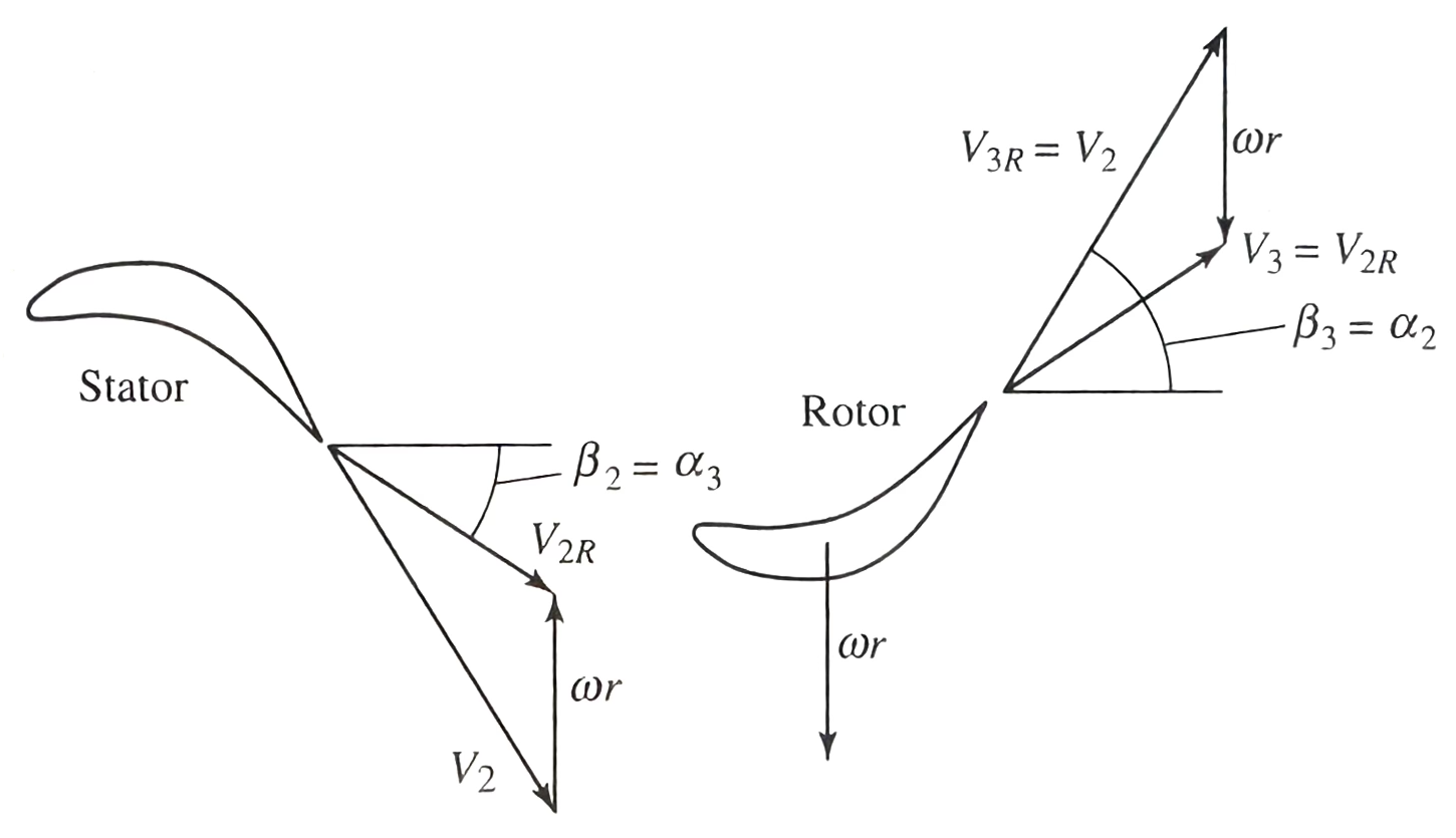
(Figure and Euqation Source: [9, p. 697])
[2] Kerrebrock, Jack L. Aircraft engines and gas turbines. MIT press, 1992.
[3] Casey, Michael, and Chris Robinson. Radial Flow Turbocompressors. Cambridge University Press, 2021.
[4] Rusch, Daniel, and Michael Casey. “The design space boundaries for high flow capacity centrifugal compressors.” Journal of turbomachinery 135.3 (2013): 031035.
[5] Cumpsty, Nicholas A. “Compressor aerodynamics.” Longman Scientific & Technical (1989).
[6] Dixon, S. Larry, and Cesare Hall. Fluid mechanics and thermodynamics of turbomachinery. Butterworth-Heinemann, 2013.
[7] Bertini, Francesco, et al. “A critical numerical review of loss correlation models and Smith diagram for modern low pressure turbine stages.” Turbo Expo: Power for Land, Sea, and Air. Vol. 55232. American Society of Mechanical Engineers, 2013.
[8] Rogers, Gordon Frederick Crichton, et al. Gas turbine theory. Pearson Higher Ed, 2017.
[9] Mattingly, Jack D. Elements of gas turbine propulsion. Vol. 1. New York: McGraw-Hill, 1996.
B-axis for 6-sided complete machining
Double tools for double MRR
Four 5-axis Turret: Kill CNC Programmers
Swiss Lathe: Assembly Line for Turning
Laser Drilling
Automation
Smart Fixturing
Ceramic Endmills
Custom Tooling
Focused ion beam-shaped microtools for ultra-precision machining
Excentric Turning
Interpolation Turning
Chatter Control
Collision Protection
AI Chip Removal
Active cooling and compensation
In-process 3D tool wear compensation
In-process surface roughness check
In-process surface probing + grinding for sub micron accuracy
“Machining” ceramics and glass
Additive + Subtractive
During IAP 2023, I had the pleasure of conducting a two-unit workshop at MIT, where students learned advanced manual and CNC machining techniques to construct a fully operational internal combustion engine in just two weeks.
I would like to extend my heartfelt gratitude to Mark Belanger, Morningside Academy for Design, Project Manus, and the Edgerton Center for their invaluable support. Additionally, a special thanks goes out to Lee Zamir and Conor McArdle for their efforts in preparing the interview.
I was reading a newsletter, which is a pretty famous one within the product management community. In this weeks’ issue, it’s said the writer is also doing angle investing now. So I looked up startups he invested in.
I can’t believe those startups are real. Because they’re just ideas in the discussions I had with schoolmates last semester. For example, I pitched an idea on 15.390 about using LiDAR to scan one’s body measurements in order to eliminate the sizing problem of online apparel shopping. And then, boom! Unspun is out there.
Another example is Cerebral. Another team on 15.390 started by building a community to let depressed patients help each other. And then they found out that a bunch of apps doing exactly the same thing are available already, so they pivot to licensed therapy, which is exactly what Cerebral offers.
And it didn’t stop there. Last October, I was having a discussion about a proposal to compete in MIT DesignX. The proposal aimed to connect the young with the elderly so that elderly could get some help and companion when they need some. But there’s one thing we didn’t figure out: how to create motives for the young to help the elderly. Papa‘s answer is the payment from the elderly’s health plan or employer.
The above examples are just from one part-time angle investor. If we look at a wider scope, there’re Modsy, Curated, AptDeco, MicroAcquire, Lawtrades, Betterleap. Every single one of these companies occurred as a startup idea in conversations I had last year. So I come to believe that everybody is being hit by apples every day, but only every few of them become Newton. What we should do is to identify ideas with market demand and start making them come true.
Be ready to be surprised by the crazy, wonderful events that will come dancing out of your past when you stir the pot of memory.
Writing about Your Life: A Journey into the Past by William Zinsser (Marlowe 2004)
I understand this point for a long time: reviewing inspires people. Actually, that’s the reason why I write blogs. So, when I came across this line from William Zinsser, I am so impressed that he could put this simple idea into such a vivid expression.
The other day, I watched this interview with a famous Chinese director, Ang Lee. I was so fascinated by the accuracy and effectiveness of his wording. For a long time, I felt feeble when trying to express myself, not matter via verbal or writing. And Lee showed me a prospect. Maybe I should take some courses in creative writing and narrative writing someday.
I’m always attracted by sci-fi works, or more specifically, space operas. What’s so-called space opera is telling stories, which originated in real life, in a space-era setting. Recently, there’s a new outstanding work available via Netflix: Space Sweepers (2021). This film talks about inequality, apartheid, and genocide.
As I am reading works by Lévi-Strauss, it comes to me that apartheid seems to be the only way to solve the problem of overpopulation so far, even in a sci-fi setting. Back to three thousand years ago, India tried to solve the population problem by the caste system. However, this is tragic for mankind. As Lévi-Strauss put it: “In the course of history, the various castes did not succeed in reaching a state in which they could remain equal because they were different.” and “When a community becomes too numerous, however great the genius of its thinkers, it can only endure by secreting enslavement.”
It appears that there are two ultimate society forms in nowadays sci-fi works. One form, featured with Elysium (2013) directed by Neill Blomkamp, is enslavement. While the others, featured with the Star Trek series, believe that space is the final and yet interminable frontier of mankind. In other words, there will always be planets where no man has gone before.
Perhaps, how we understand the problem of overpopulation is just as limited as how Malthus understand it in the 1800s. But, anyway, it is just a little depressing that sci-fi works—representing the boundary of human imagination—reach the same conclusion as what thinkers in India came to three thousand years ago.
It has been three months since the first time I tried to write about this spot on planet earth. It seems that Aranya carries too much meaning for me, that every time I tried to order my thoughts, I accomplished nothing but becoming effusive. Until recently.
Last week, I came across some lines from Claude Lévi-Strauss. It feels like Thanos snapped his fingers and my confusion vanished. I share a similar dilemma about Aranya as Claude feels about mountains: on the one hand, I value the solitude of it, and on the other hand, the solitude may cause the termination of Aranya.
For some years past, this preference has taken the form of a jealous passion. I hated who those shared my predilection, for they were a menace to the solitude I value so highly; and I despised those others for whom mountains meant merely physical exhaustion and a constricted horizon and who were, for that reason, unable to share in my emotions. The only thing that would have satisfied me would have been for the entire world to admit to the superiority of mountains and grant me the monopoly of their enjoyment.
Lévi-Strauss, C. (1992). Tristes tropiques (1955). Trans. John and Doreen Weightman. London: Penguin Books, 333.
In other words, it’s similar to the Arc Reactor for Tony Stark. It is the reactor that keeps Stark alive while the palladium within the reactor is poisoning him.
This is when I fell in love with Aranya. It’s very much like a scene in Oblivion: after a long period of time, humans became barely extinct. Just as Claude wrote in another chapter of the book I quoted above, the signs of the existence of human beings mark out, more clearly than if humans had not been there, the extreme limit that they have attempted to cross. Great nature placates the rebellion of humans and quells my turbulence.
I’m also a diehard fan of open water. Ripples on the surface make him alive. And he’s always here, listening. There’s a peaceful lake on my college campus. Without doubts, that’s the place for the inner me. Every time I approach the lake, the clamour in my mind fades away. It’s like a gigantic jar, purged and stored all my feelings——happy, sad, and everything in between. I always characterize the lake as a pensive old man. Not the style of The Old Man and the Sea, but more like Yoda.
In addition, Aranya is not only the certainty of space but also a state of mind. I’ve been super busy for the past year. And as far as I could tell, the coming one would not be of much leisure. Therefore, some time for simply wandering around is such a luxury for me. In the space opera Star Trek: The Next Generation, there’s some discussion about what makes humans different. Or, in other words, if a single feature of human is picked as the representative of mankind, which one would occupy the place of honour? The answer proposed by scriptwriters is curiosity. And I kind of agree with this one. Sir Ken Robinson once said: There are two types of people in this world: those who divide the world into two types and those who do not. Continuing this manner, I would like to divide the pursuit of curiosity into two kinds: those which require teamwork and those which do not. Throughout the last year, I’m offered some wonderful chances to collaborate with brilliant collaborators. A lost chance never returns. So, collaborations dominated my time. By and large, Aranya becomes the very only and dilapidated refuge for the private part of curiosity.
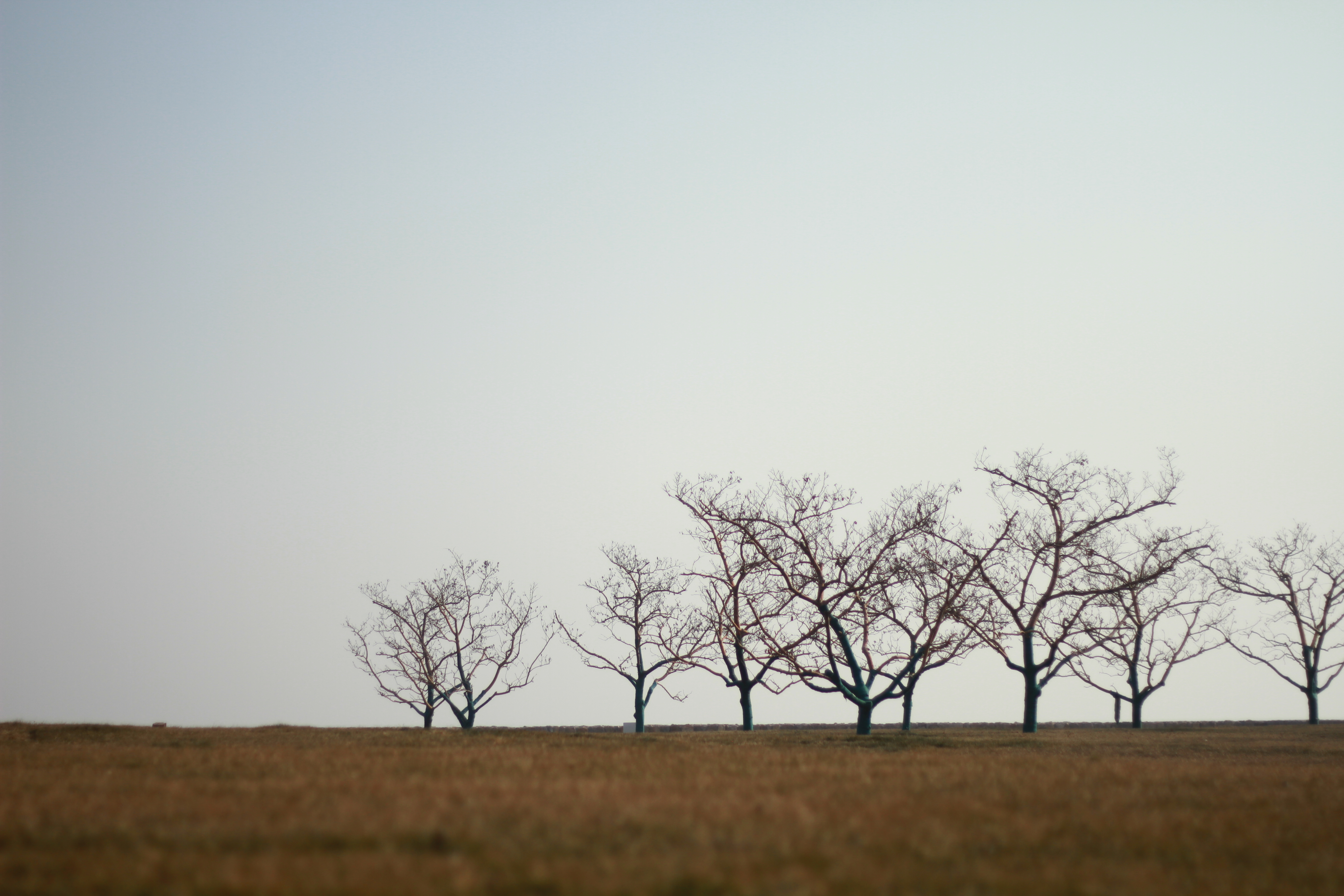
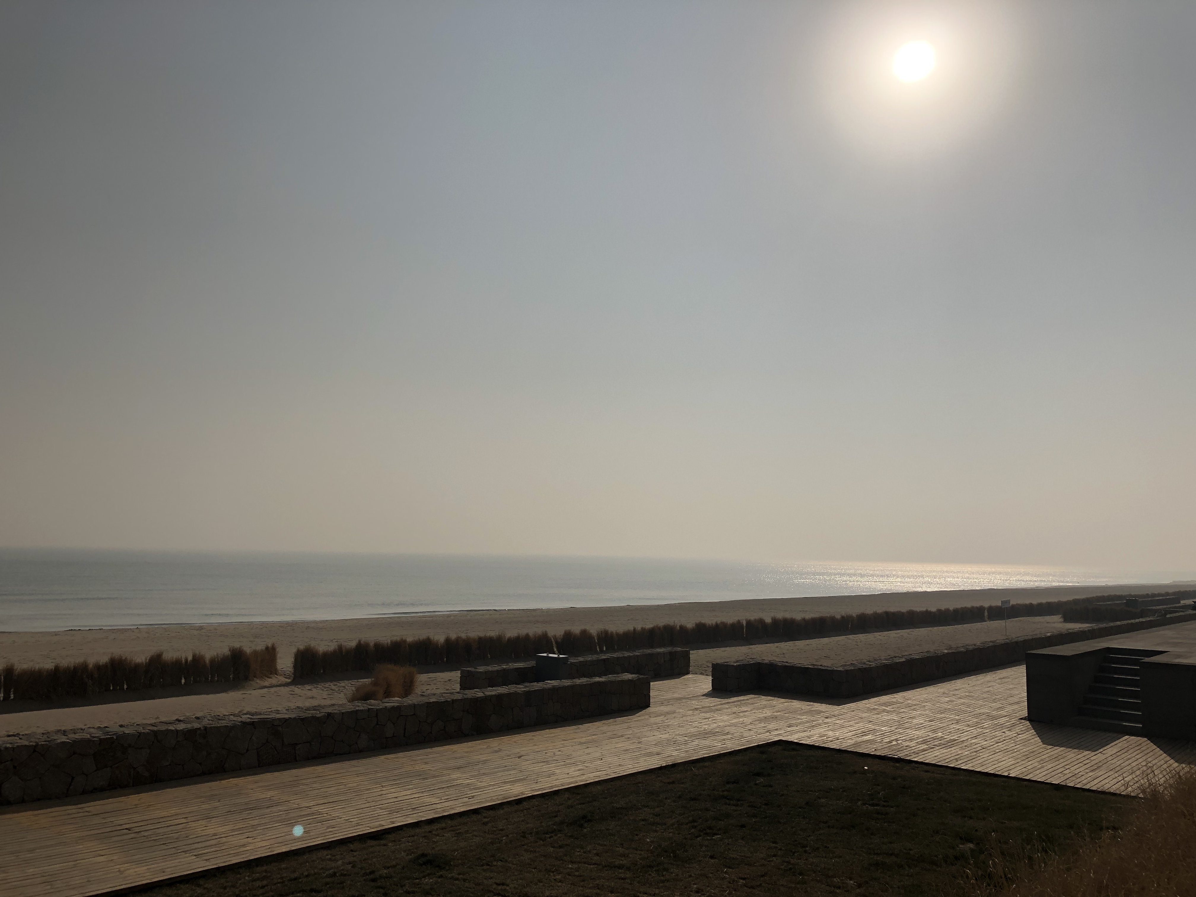
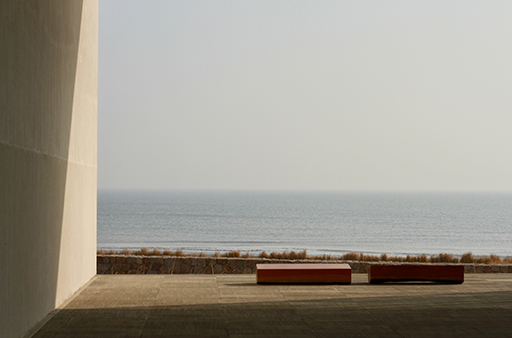
Every time I plan to spend some time at Aranya, I agonize. I’m so afraid that it may perish. Every visit I paid might be the valediction. I took the beginning picture of this article on my first visit to Aranya. And on my second trip here, it’s gone, encroached by a construction site. The following ones were taken during my first and second visits. Unfortunately, the spot disappeared before my third visit, with no trace. I hate what’s happening out there, but there’s nothing I can do except presenting my raw passion.
How this is gonna end? Maybe Aranya will still be there long after my death, while it’s entirely possible that it’s gone by tomorrow. I guess the only thing I could do and what I’m doing is that enjoy every moment with Aranya until the termination of either one of us.
Who knows where the road will lead us?
Sinatra, F. (1957). All the Way.
Only a fool would say
But if you’ll let me love you
It’s for sure I’m gonna love you
All the way