1. Compressor Impeller Design

1.1. Design Requirements

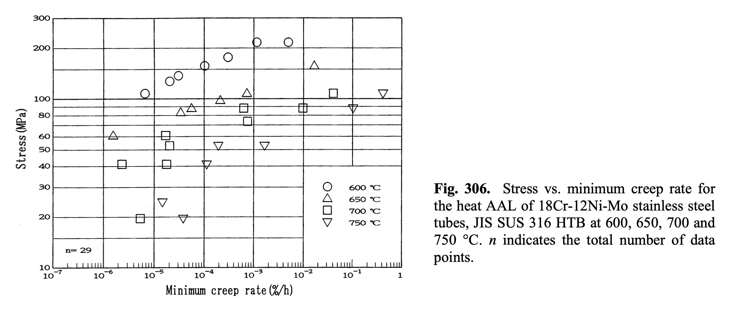
The design target for the second generation engine is a power output of 10 kW with a thermal efficiency, defined as the equation below, of more than 10%. $$ \eta_\textrm{thermal}=\frac{\text{net power out}}{\text{fuel mass flow rate} \times \text{fuel lower heating value}}=\frac{(1+f)c_p^c T_{t4} \eta_T (1-\Pi^{\frac{1-\gamma^c}{\gamma^c}}) – \frac{c_p^a T_{0}}{\eta_C} (\Pi^{\frac{\gamma^a-1}{\gamma^a}}-1)}{f h_c} $$ For ease of fabrication, the turbine material is selected to be 316 Stainless Steel, which has a yield strength of more than 120 MPa at 650 C. For long term exposure to heat, it has less than 0.1% elongation at 1000 hours at 85 MPa at 650 C [1]. This decision leads to $T_{t4}=650 \text{ C} \approx 920 \text{ K}$.

The second generation engine is expected to have a radial compressor and an axial turbine. A conservative estimation of compressor efficiency and turbine efficiency is made: $\eta_c = 0.8$, $\eta_t = 0.85$.

The fuel is selected to be propane, which has a lower heating value of $h_c = 4.64 \times 10^7$ J / kg.

Some common assumptions are made to the rest of the variables:

1. $c_p^a = 1004$ J⋅kg$^{−1}$⋅K$^{−1}$
2. $c_p^c = 1200$ J⋅kg$^{−1}$⋅K$^{−1}$
3. $\gamma^a = 1.4$
4. $\gamma^c = 1.3$
5. Compressor Inlet Tempurature $T_0 = 298$ K

Now, plotting $\eta_\textrm{thermal}$ vs pressure ratio $\Pi$ using this code, we have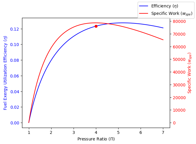

The pressure ratio is set to 4.0 to maximize specific work. At this design point, specific work is 78,700 J/kg and $\eta_\textrm{thermal}$ is predicted to be 12.3%. Fuel-to-air ratio at design point is calculated as $$f = \frac{c^c_p T_{t4} – c_p^a T_{t3}}{h_c-c_p^c T_{t4}}= 1.376%$$, where $T_{t3}$ is calculated as $$T_{t3} = T_0 (\frac{\Pi^{(\gamma^a-1)/\gamma^a}-1}{\eta_c}+1) = 479 \text{ K}$$.

According to specific work, in order to have 10 kW output, we need a massflow rate of 0.127 kg/s. This is less than half of the massflow rate designed for Gentoo. Due to a previous calculation error, a massflow rate of 0.128 kg/s will be used for the rest of the documents.

Aiming for a compact size, to get to this kind of pressure ratio is almost required to go with hybrid or full ceramic bearings. A very cost effective choice is this hybrid ceramic bearing from GRW, which is rated at 160,000 rpm. So, let’s set the upper limit of spool speed to 160,000 rpm. Other bearing choices for this speed would be: CXMC-1980 and HY KH 61900 C TA.

Due to the limitation of fabrication equipment, we can process rod stock with a diameter up to 200 mm. Say, half of the diameter is reserved for diffuser, the impeller diameter $D_w \leq 100$ mm.

As a summary, the following design requirements are selected for the impeller:

• Compressor Pressure Ratio $\Pi_c = 4.0$
• Isentropic Efficiency $\eta_c = 80%$ (Polytropic Efficiency $\eta_{c,\text{ploy}}=83.5%$)
• Massflow Rate $\dot{m} = 0.128$ kg/s
• Spool Speed $\omega \leq$ 160,000 rpm
• Impeller Diameter $D_2 \leq 100$ mm

1.2. Flow Coefficient

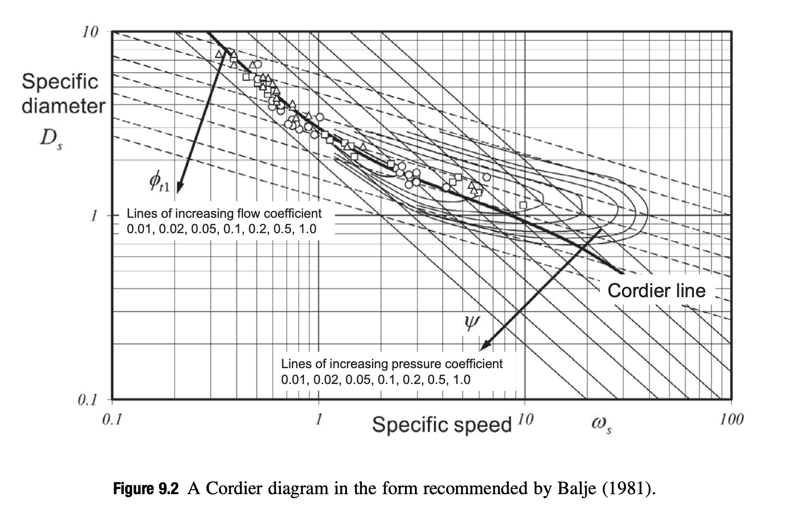
According to [3, p. 326], it is common to pick a flow coefficient in the range of $0.07 \leq \phi_{t1} \leq 0.10$. See the figure below (quoted from the book) for the relationship. Originally, a $\phi_{t1} = 0.09$ is selected for highest efficiency. But later, $\phi_{t1} = 0.057$ is used due the speed limitation imposed by bearings.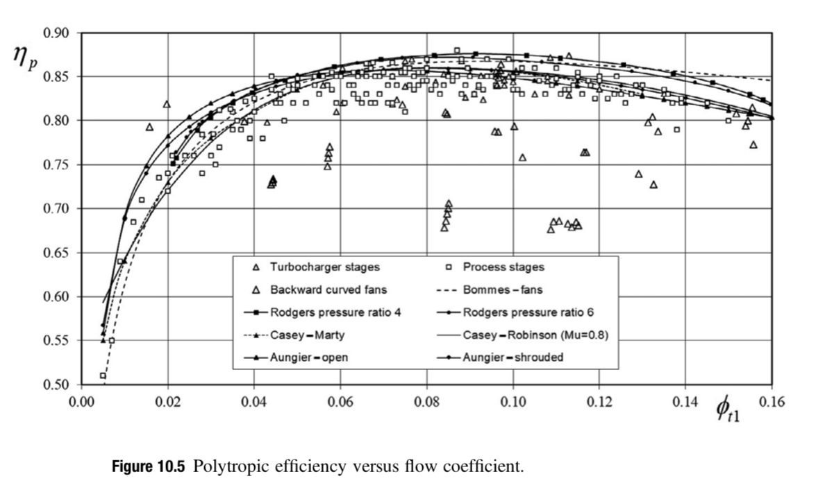

1.3. Work Coefficient

According to multiple source, it is common to have a work coefficient around 0.7 for higher efficiency and lower tip speed. Therefore, work coefficient is choosen to be $\lambda = \frac{c_{u2}}{u_2} = \frac{\Delta h_t}{(\omega R_2)^2} = \frac{\omega \Delta (rc\theta)}{(\omega R_2)^2} = 0.7$.

1.4. Sizing and Velocities

According to [3, p. 330], We have:

$$ M_{u2}^2=\frac{\Pi^{\frac{\gamma-1}{\eta_{\text{ploy}} \cdot \gamma}}-1}{(\gamma-1)\lambda} $$

According to the definition of polytropic efficiency and assumption for ideal gas, we have

$$ \eta_c = \frac{\Pi^{(\gamma-1)/\gamma}-1}{\Pi^{(\gamma-1)/(\eta_{\text{poly}}\gamma)}-1} $$

Therefore, we have

$$ M_{u2}^2 = \frac{\Pi^{(\gamma-1)/\gamma}-1}{\eta_c(\gamma-1)\lambda} \approx 2.17 $$

and

$$ M_{u2} \approx 1.473 $$

Therefore,

$$ u_2=M_{u2}\sqrt{\gamma \text{R} T_{0}} \approx 510 \text{ m/s} $$

This result matches the prediction in [3, p. 267]. The Diameter of the impeller can be then calculated as (from [3, p. 255]):

$$ D_2 = \sqrt{\frac{\dot{m}}{\rho_{t1}u_2\phi_{t1}}} $$

When using $\rho_{t1}=1.18$ kg/m$^3$, we have $D_2$ = 61.1 mm. The speed is then calculated to be $\omega$ = 159,315 rpm. Both $D_2$ and $\omega$ satisfy our design requirements.

Then the relative Mach number at the inlet tip can be calculated as

$M_{w1}=\frac{M_{u2}(\frac{3.2 \phi_{t1}}{k})^{0.36}}{1-0.15M_{u2}(0.45+\frac{\phi_{t1}}{k})} = 0.931$, where impeller inlet shape factor $k = 1-(\frac{r_{1h}}{r_{1c}})^2 = 0.91$ is assumed. Equation source: [3, p. 353].

Then optimal flow inlet angle can be calculated as $\beta_{1c}=cos^{-1}(\frac{\sqrt{3+\gamma M_{w1}^2 + 2 M_{w1}} – \sqrt{3+ \gamma M_{w1}^2-2M_{w1}}}{2M_{w1}})=1.047 \text{ rad}= 60.0 ^\circ $. Source: [3, p 348].

The inlet diameter ratio can be then calculated as $\frac{D_{1c}}{D_2}= \frac{M_{w1}\sin (\beta_{1c})}{M_{u2}\sqrt{1+\frac{\gamma -1}{2}M_{w1}^2 \cos ^2{\beta_{1c}}}}=0.536 $ . Source: [4].

Then we know our impeller eye diameter $D_{1c}=32.8 $ mm. After that, inlet hub diameter can be calculated using inlet shape diameter $k$, $D_{1h}=D_{1c}\sqrt{1-k}=9.8 $ mm.

Impeller relative velocity at the casing can be then calculated as $w_{1c} = u_2 \frac{2D_{1c}}{\sqrt{3}D_2} = 316 $ m/s.

A de Haller number of $\text{DH} = 0.6$ is choose for medium diffusion. Then $w_2= \text{DH} \cdot w_{c1}=190$ m/s.

By ultilizating, outlet velocity triangle, $\frac{w_{u2}-c_s}{c_{m2}}=\tan \beta_2’ $ and the Wiesner correlation $\frac{c_s}{u_2}=\frac{\sqrt{\cos \beta_2’}}{Z^{0.7}}$ where Z is the number of blades at outlet, we can solve for the outlet backsweep angle $\beta_2’=26.8 ^\circ$ if $Z = 10$, or $\beta_2’=32.0 ^\circ$ if $Z = 12$, or $\beta_2’=35.5 ^\circ$ if $Z = 14$. In order to have a high efficiency and side operating range, $Z = 12$ is chosen for a backsweep angle of $\beta_2’=32.0 ^\circ$.

1.5. Velocity Triangles

1.5.1 Inlet Velocity Triangle

(Figure Source: [3])

• $\omega = $ 159,315 rpm
• $\beta_{c1}=1.047 \text{ rad}= 60.0 ^\circ$
• $u_{c1} = 273.6$ m/s
• $c_{m1}=c_1=158.1 $ m/s
• $w_{c1}=316$ m/s

1.5.2 Outlet Velocity Triangle

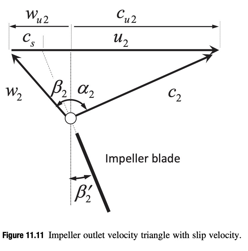
(Figure & Estimation Source: [3]. See section 11.6.6 in this book for outlet velocity triangle design process.)

• $u_2=510$ m/s
• $c_{u2}=\lambda u_2=357 $ m/s
• $w_{u2}=u_2-c_{u2}=153$ m/s
• $w_2 = 190$ m/s
• $c_{m2}=\sqrt{w_2^2-w_{u2}^2}=112.7 $ m/s
• $\phi_2=\frac{c_{m2}}{u_2}= 0.221$
• $c_2 = \sqrt{c_{m2}^2+c_{u2}^2}=374.4 $ m/s
• $\alpha_2 = \sin^{-1}(\frac{c_{u2}}{c_2}) = 1.265 \text{ rad} = 72.5 ^\circ $
• $\beta_2 = \sin^{-1}(\frac{w_{u2}}{w_2})=0.936 \text{ rad} = 53.6 ^\circ$
• $\beta_2’= 0.559 \text{ rad} = 32.0 ^\circ $
• $c_s = u_2\frac{\sqrt{\cos \beta_2’}}{Z^{0.7}}=82.5$ m/s

1.6. Verification

1.6.1 Pressure Rise Coefficient

The pressure rise coefficient $\psi=\frac{\Delta h_0}{U^2}=\frac{\Delta p}{\rho \omega^2D_2^2}=\lambda\eta_s=0.56$. According to [3, p. 285], an optimal value of $\psi=0.55 \pm 0.05$ is recommended. Our $\psi$ is in the optimal range.

1.6.1 Specific Speed & Specific Diameter

Then specific speed is calculated as $\omega_s=2\frac{\phi_{t1}^{1/2}}{\psi^{3/4}}=0.7376$, while the specific diameter is calculated as $D_s = \frac{\psi^{1/4}}{\phi_{t1}^{1/2}} = 3.623 $.

According to a cordier diagram plotted in [3, p. 291], our design point is very close to the Cordier Line (max efficiency).

2. Turbine Design

An axial turbine configuration rather than radial turbine is selected for higher efficiency. Since the pressure ratio of compressor is only 4, single stage axial turbine should be able to do the work with fairly high efficiency.

2.1. Flow Coefficient, Work Coefficient, and Degree of Reaction

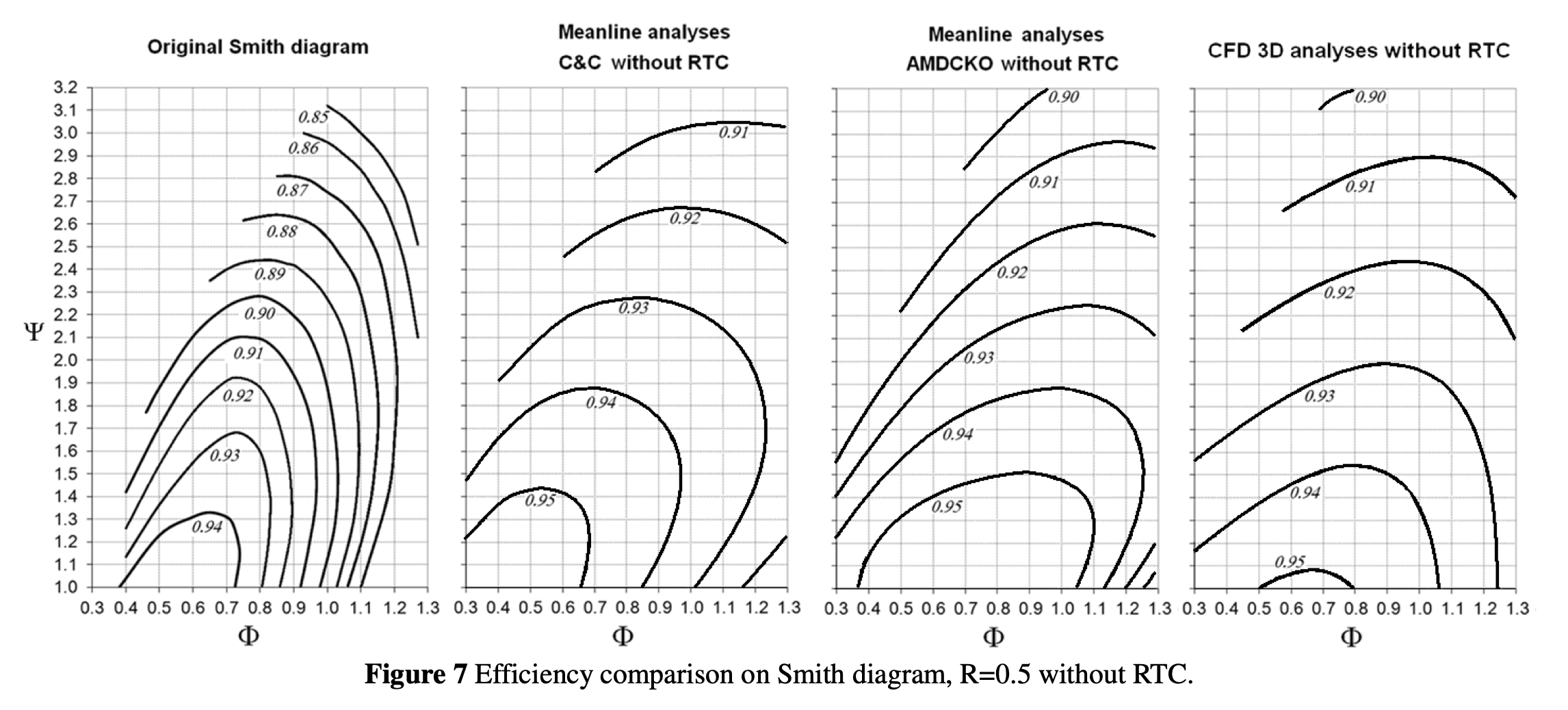
Multiple versions of Smith Charts are avaliable to help select these parameters. The following values are selected for maximum efficiency:

• Work Coefficient $\Psi = 1.2 = \frac{\Delta h_0}{U^2} = \frac{\Delta c_{\theta}}{U}$
• Degree of Reaction $\text{R} = 0.5 = \frac{h_2-h_3}{h_1-h_3} \approx \frac{p_2-p_3}{p_1-p_3}$

The following parameter is a bit away from optimal due to the stress consideration imposed by turbine material:

• Flow Coefficient $\phi = 0.90 = \frac{c_x}{U}$

The defination of these parameter can be found at [6, p. 122-123].

A recommanded paper about Smith Chart can be found in [7]. Here’s one version of Smith Chart from this paper:

2.2. Turbine-Compressor Matching

The turbine will be installed on the same shaft with compressor impeller, and therefore $\omega_t = \omega_c = $ 159,315 rpm.

The turbine should be able to supply the right amount of power to run compressor. From the compressor design, the compressor need a specific work of

$$ W_{sp}= \frac{c_p^a T_{0}}{\eta_c} (\Pi^{\frac{\gamma^a-1}{\gamma^a}}-1)= \text{181,757 J/kg} $$

Assuming there’s a 1% mechanical loss, suggested in [8, p. 65], the turbine needs to extract $W_{sp}= $ 183,593 J/kg. Therefore, the power needed to run the compressor is $23.5$ kw.

Then the pressure ratio needed for the turbine to provide enough power can be calculated as $$ \Pi_{\text{turbine}}=(1-\frac{W_{sp}}{(1+f)c_p^c T_{t4} \eta_T })^{\frac{\gamma^c}{1-\gamma^c}} = 2.53 $$

2.3. Blade Speed, Height, and Mean Radius

According to [8, p. 134], minimal blade tip speed can be calculated as $$ U \geq \sqrt{\frac{\dot{W}}{\dot{m}\Psi}}=391.1 \text{ m/s} $$ Using air density $\rho=1.53$ kg/m$^3$ at 4 atm pressure and 650 C, the annulus area can be calculated as $$ A_x=\frac{\dot{m}}{\rho\phi U}=237.7 \text{ mm}^2 $$ By using the equation $$ A_x=\pi r_t^2(1-(\frac{r_h}{r_t})^2) $$ and the following equation from [8, p. 152]. which estimates centrifugal stress $$ \frac{\sigma_c}{\rho_m}=\frac{(\omega r_t)^2}{2}(1-(\frac{r_h}{r_t})^2) $$ We can estimates the centrifugal stress (assuming $\rho_m$ = 7980 kg/m$^3$, $\omega=159315 \text{ rpm}=16683.4 \text{ rad/s}$) $$ \sigma_c = \frac{\rho_m\omega^2A_x}{2\pi}=84 \text{ MPa} $$ Which is looks good for to satisfty creep resistance requirement.

The blade mean radius can be calculated as $r_m=\frac{U}{\omega}=23.4$ mm, and the blade height can be then calculated as $$ r_t-r_h=H\approx \frac{\dot{m}}{\rho \phi U 2 \pi r_m}=1.61 \text{ mm} $$ Therefore, we have turbine hub radius $r_h = 21.8$ mm, and turbine tip radius $r_t=25$ mm.

2.4. Velocity Triangles

$\Psi = \frac{\Delta v}{\omega r} = 2\phi \tan \alpha_2-1=2\phi \tan \beta_3-1$, and therefore we have $$ \alpha_2 = \beta_3 = \tan^{-1}(\frac{\Psi+1}{2\phi})=0.885 \text{ rad}=50.7 ^\circ $$ and because of $\tan \beta_3 – \tan \beta_2 = \frac{\omega r}{u_2} = \frac{1}{\phi}$ $$ \alpha_3 = \beta_2 = \tan^{-1}(\frac{\Psi-1}{2\phi})=0.111 \text{ rad}=6.3 ^\circ $$ from previous calculation, we have $\omega r = U = 391.1 \text{ m/s}$ and $c_x=\phi U = 352.0 \text{ m/s}$, and therefore we have $$ V_{2R} = V_3 = \frac{c_x}{\cos \beta_2} = 354.2 \text{ m/s} $$

$$ V_2 = V_{3R}=\sqrt{c_x^2 + (c_x\tan \beta_2 + U)^2} = 556.0 \text{ m/s} $$

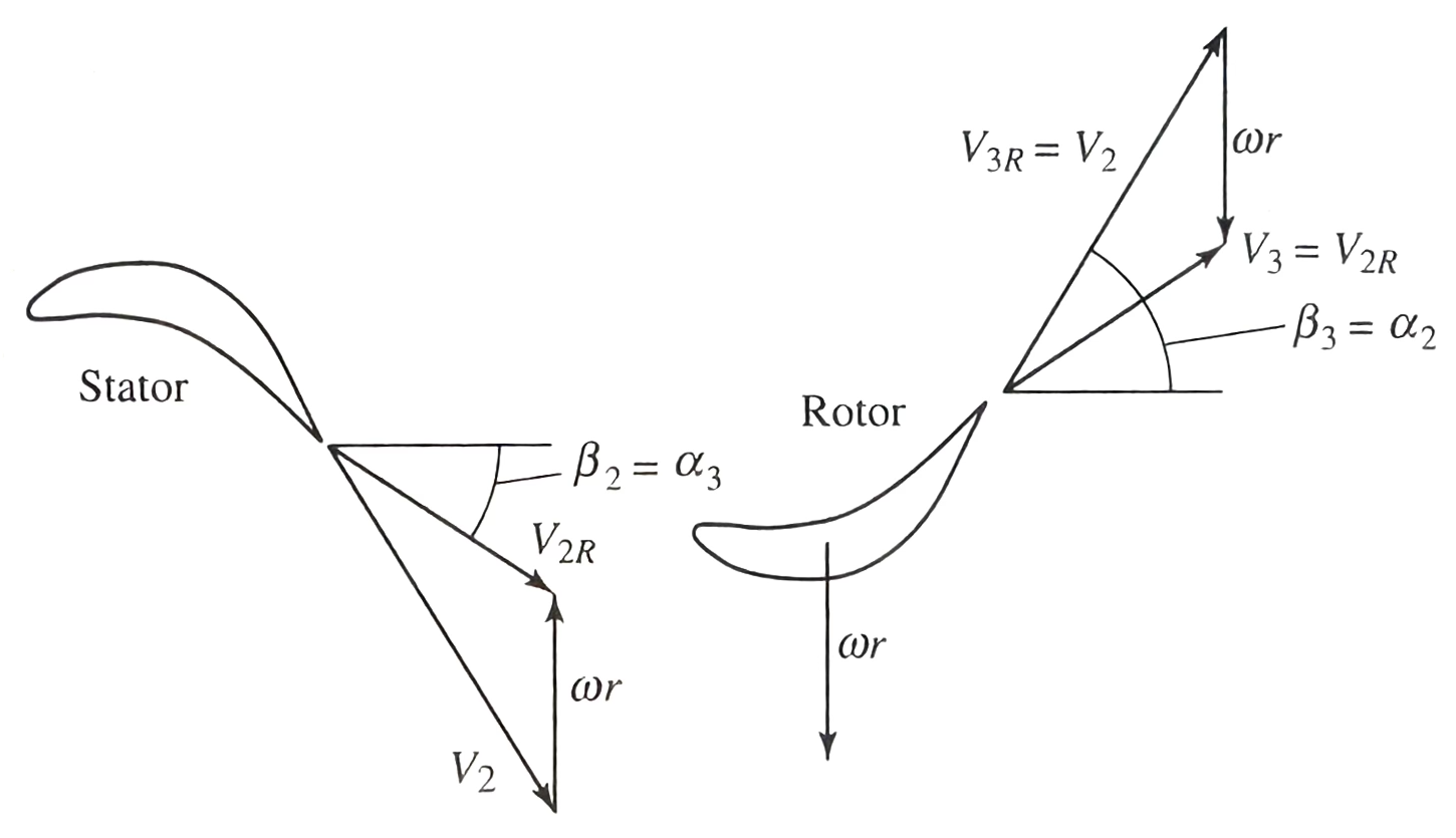
(Figure and Euqation Source: [9, p. 697])

Reference

[1] Yagi, K., et al. “Creep properties of heat resistant steels and superalloys.” Landolt Bornstein numerical data & functional relationships in science & technology, Springer, 2nd editions(2004)

[2] Kerrebrock, Jack L. Aircraft engines and gas turbines. MIT press, 1992.

[3] Casey, Michael, and Chris Robinson. Radial Flow Turbocompressors. Cambridge University Press, 2021.

[4] Rusch, Daniel, and Michael Casey. “The design space boundaries for high flow capacity centrifugal compressors.” Journal of turbomachinery 135.3 (2013): 031035.

[5] Cumpsty, Nicholas A. “Compressor aerodynamics.” Longman Scientific & Technical (1989).

[6] Dixon, S. Larry, and Cesare Hall. Fluid mechanics and thermodynamics of turbomachinery. Butterworth-Heinemann, 2013.

[7] Bertini, Francesco, et al. “A critical numerical review of loss correlation models and Smith diagram for modern low pressure turbine stages.” Turbo Expo: Power for Land, Sea, and Air. Vol. 55232. American Society of Mechanical Engineers, 2013.

[8] Rogers, Gordon Frederick Crichton, et al. Gas turbine theory. Pearson Higher Ed, 2017.

[9] Mattingly, Jack D. Elements of gas turbine propulsion. Vol. 1. New York: McGraw-Hill, 1996.